Shortest Paths
Overview
The shortest path problem is a classic problem in mathematics and computer science with applications in
- Economics (sequential decision making, analysis of social networks, etc.)
- Operations research and transportation
- Robotics and artificial intelligence
- Telecommunication network design and routing
- etc., etc.
Variations of the methods we discuss in this lecture are used millions of times every day, in applications such as
- Google Maps
- routing packets on the internet
For us, the shortest path problem also provides a nice introduction to the logic of dynamic programming.
Dynamic programming is an extremely powerful optimization technique that we apply in many lectures on this site.
The only scientific library we’ll need in what follows is NumPy:
import numpy as np
Outline of the Problem
The shortest path problem is one of finding how to traverse a graph from one specified node to another at minimum cost.
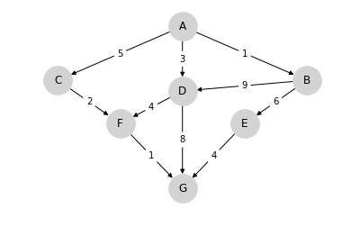
Consider the following graph

We wish to travel from node (vertex) A to node G at minimum cost
- Arrows (edges) indicate the movements we can take.
- Numbers on edges indicate the cost of traveling that edge.
(Graphs such as the one above are called weighted directed graphs)
Possible interpretations of the graph include
- Minimum cost for supplier to reach a destination.
- Routing of packets on the internet (minimize time).
- Etc., etc.
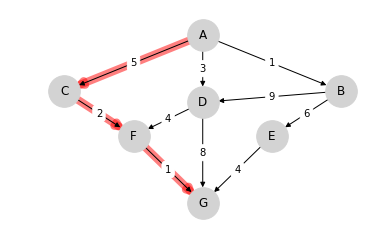
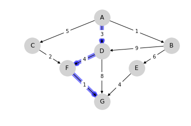
For this simple graph, a quick scan of the edges shows that the optimal paths are
- A, C, F, G at cost 8

- A, D, F, G at cost 8

Finding Least-Cost Paths
For large graphs, we need a systematic solution.
Let $ J(v) $ denote the minimum cost-to-go from node $ v $, understood as the total cost from $ v $ if we take the best route.
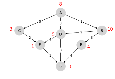
Suppose that we know $ J(v) $ for each node $ v $, as shown below for the graph from the preceding example

Note that $ J(G) = 0 $.
The best path can now be found as follows
- Start at node $ v = A $
- From current node $ v $, move to any node that solves
$$ \min_{w \in F_v} \{ c(v, w) + J(w) \} \tag{1} $$
where
- $ F_v $ is the set of nodes that can be reached from $ v $ in one step.
- $ c(v, w) $ is the cost of traveling from $ v $ to $ w $.
Hence, if we know the function $ J $, then finding the best path is almost trivial.
But how can we find the cost-to-go function $ J $?
Some thought will convince you that, for every node $ v $, the function $ J $ satisfies
$$ J(v) = \min_{w \in F_v} \{ c(v, w) + J(w) \} \tag{2} $$
This is known as the Bellman equation, after the mathematician Richard Bellman.
The Bellman equation can be thought of as a restriction that $ J $ must satisfy.
What we want to do now is use this restriction to compute $ J $.
Solving for Minimum Cost-to-Go
Let’s look at an algorithm for computing $ J $ and then think about how to implement it.
The Algorithm
The standard algorithm for finding $ J $ is to start an initial guess and then iterate.
This is a standard approach to solving nonlinear equations, often called the method of successive approximations.
Our initial guess will be
$$ J_0(v) = 0 \text{ for all } v \tag{3} $$
Now
- Set $ n = 0 $
- Set $ J_{n+1} (v) = \min_{w \in F_v} \{ c(v, w) + J_n(w) \} $ for all $ v $
- If $ J_{n+1} $ and $ J_n $ are not equal then increment $ n $, go to 2
This sequence converges to $ J $.
Although we omit the proof, we’ll prove similar claims in our other lectures on dynamic programming.
Implementation
Having an algorithm is a good start, but we also need to think about how to implement it on a computer.
First, for the cost function $ c $, we’ll implement it as a matrix $ Q $, where a typical element is
$$ Q(v, w) = \begin{cases} & c(v, w) \text{ if } w \in F_v \\ & +\infty \text{ otherwise } \end{cases} $$In this context $ Q $ is usually called the distance matrix.
We’re also numbering the nodes now, with $ A = 0 $, so, for example
$$ Q(1, 2) = \text{ the cost of traveling from B to C } $$For example, for the simple graph above, we set
from numpy import inf

Q = np.array([[inf, 1,   5,   3,   inf, inf, inf],
              [inf, inf, inf, 9,   6,   inf, inf],
              [inf, inf, inf, inf, inf, 2,   inf],
              [inf, inf, inf, inf, inf, 4,   8],
              [inf, inf, inf, inf, inf, inf, 4],
              [inf, inf, inf, inf, inf, inf, 1],
              [inf, inf, inf, inf, inf, inf, 0]])
Notice that the cost of staying still (on the principle diagonal) is set to
- np.inf for non-destination nodes — moving on is required.
- 0 for the destination node — here is where we stop.
For the sequence of approximations $ \{J_n\} $ of the cost-to-go functions, we can use NumPy arrays.
Let’s try with this example and see how we go:
nodes = range(7)                              # Nodes = 0, 1, ..., 6
J = np.zeros_like(nodes, dtype=np.int)        # Initial guess
next_J = np.empty_like(nodes, dtype=np.int)   # Stores updated guess

max_iter = 500
i = 0

while i < max_iter:
    for v in nodes:
        # minimize Q[v, w] + J[w] over all choices of w
        lowest_cost = inf
        for w in nodes:
            cost = Q[v, w] + J[w]
            if cost < lowest_cost:
                lowest_cost = cost
        next_J[v] = lowest_cost
    if np.equal(next_J, J).all():
        break
    else:
        J[:] = next_J   # Copy contents of next_J to J
        i += 1

print("The cost-to-go function is", J)
This matches with the numbers we obtained by inspection above.
But, importantly, we now have a methodology for tackling large graphs.
Exercises
Exercise 1
The text below describes a weighted directed graph.
The line node0, node1 0.04, node8 11.11, node14 72.21 means that from node0 we can go to
- node1 at cost 0.04
- node8 at cost 11.11
- node14 at cost 72.21
No other nodes can be reached directly from node0.
Other lines have a similar interpretation.
Your task is to use the algorithm given above to find the optimal path and its cost.
Note: You will be dealing with floating point numbers now, rather than
integers, so consider replacing np.equal() with np.allclose().
%%file graph.txt
node0, node1 0.04, node8 11.11, node14 72.21
node1, node46 1247.25, node6 20.59, node13 64.94
node2, node66 54.18, node31 166.80, node45 1561.45
node3, node20 133.65, node6 2.06, node11 42.43
node4, node75 3706.67, node5 0.73, node7 1.02
node5, node45 1382.97, node7 3.33, node11 34.54
node6, node31 63.17, node9 0.72, node10 13.10
node7, node50 478.14, node9 3.15, node10 5.85
node8, node69 577.91, node11 7.45, node12 3.18
node9, node70 2454.28, node13 4.42, node20 16.53
node10, node89 5352.79, node12 1.87, node16 25.16
node11, node94 4961.32, node18 37.55, node20 65.08
node12, node84 3914.62, node24 34.32, node28 170.04
node13, node60 2135.95, node38 236.33, node40 475.33
node14, node67 1878.96, node16 2.70, node24 38.65
node15, node91 3597.11, node17 1.01, node18 2.57
node16, node36 392.92, node19 3.49, node38 278.71
node17, node76 783.29, node22 24.78, node23 26.45
node18, node91 3363.17, node23 16.23, node28 55.84
node19, node26 20.09, node20 0.24, node28 70.54
node20, node98 3523.33, node24 9.81, node33 145.80
node21, node56 626.04, node28 36.65, node31 27.06
node22, node72 1447.22, node39 136.32, node40 124.22
node23, node52 336.73, node26 2.66, node33 22.37
node24, node66 875.19, node26 1.80, node28 14.25
node25, node70 1343.63, node32 36.58, node35 45.55
node26, node47 135.78, node27 0.01, node42 122.00
node27, node65 480.55, node35 48.10, node43 246.24
node28, node82 2538.18, node34 21.79, node36 15.52
node29, node64 635.52, node32 4.22, node33 12.61
node30, node98 2616.03, node33 5.61, node35 13.95
node31, node98 3350.98, node36 20.44, node44 125.88
node32, node97 2613.92, node34 3.33, node35 1.46
node33, node81 1854.73, node41 3.23, node47 111.54
node34, node73 1075.38, node42 51.52, node48 129.45
node35, node52 17.57, node41 2.09, node50 78.81
node36, node71 1171.60, node54 101.08, node57 260.46
node37, node75 269.97, node38 0.36, node46 80.49
node38, node93 2767.85, node40 1.79, node42 8.78
node39, node50 39.88, node40 0.95, node41 1.34
node40, node75 548.68, node47 28.57, node54 53.46
node41, node53 18.23, node46 0.28, node54 162.24
node42, node59 141.86, node47 10.08, node72 437.49
node43, node98 2984.83, node54 95.06, node60 116.23
node44, node91 807.39, node46 1.56, node47 2.14
node45, node58 79.93, node47 3.68, node49 15.51
node46, node52 22.68, node57 27.50, node67 65.48
node47, node50 2.82, node56 49.31, node61 172.64
node48, node99 2564.12, node59 34.52, node60 66.44
node49, node78 53.79, node50 0.51, node56 10.89
node50, node85 251.76, node53 1.38, node55 20.10
node51, node98 2110.67, node59 23.67, node60 73.79
node52, node94 1471.80, node64 102.41, node66 123.03
node53, node72 22.85, node56 4.33, node67 88.35
node54, node88 967.59, node59 24.30, node73 238.61
node55, node84 86.09, node57 2.13, node64 60.80
node56, node76 197.03, node57 0.02, node61 11.06
node57, node86 701.09, node58 0.46, node60 7.01
node58, node83 556.70, node64 29.85, node65 34.32
node59, node90 820.66, node60 0.72, node71 0.67
node60, node76 48.03, node65 4.76, node67 1.63
node61, node98 1057.59, node63 0.95, node64 4.88
node62, node91 132.23, node64 2.94, node76 38.43
node63, node66 4.43, node72 70.08, node75 56.34
node64, node80 47.73, node65 0.30, node76 11.98
node65, node94 594.93, node66 0.64, node73 33.23
node66, node98 395.63, node68 2.66, node73 37.53
node67, node82 153.53, node68 0.09, node70 0.98
node68, node94 232.10, node70 3.35, node71 1.66
node69, node99 247.80, node70 0.06, node73 8.99
node70, node76 27.18, node72 1.50, node73 8.37
node71, node89 104.50, node74 8.86, node91 284.64
node72, node76 15.32, node84 102.77, node92 133.06
node73, node83 52.22, node76 1.40, node90 243.00
node74, node81 1.07, node76 0.52, node78 8.08
node75, node92 68.53, node76 0.81, node77 1.19
node76, node85 13.18, node77 0.45, node78 2.36
node77, node80 8.94, node78 0.98, node86 64.32
node78, node98 355.90, node81 2.59
node79, node81 0.09, node85 1.45, node91 22.35
node80, node92 121.87, node88 28.78, node98 264.34
node81, node94 99.78, node89 39.52, node92 99.89
node82, node91 47.44, node88 28.05, node93 11.99
node83, node94 114.95, node86 8.75, node88 5.78
node84, node89 19.14, node94 30.41, node98 121.05
node85, node97 94.51, node87 2.66, node89 4.90
node86, node97 85.09
node87, node88 0.21, node91 11.14, node92 21.23
node88, node93 1.31, node91 6.83, node98 6.12
node89, node97 36.97, node99 82.12
node90, node96 23.53, node94 10.47, node99 50.99
node91, node97 22.17
node92, node96 10.83, node97 11.24, node99 34.68
node93, node94 0.19, node97 6.71, node99 32.77
node94, node98 5.91, node96 2.03
node95, node98 6.17, node99 0.27
node96, node98 3.32, node97 0.43, node99 5.87
node97, node98 0.30
node98, node99 0.33
node99,
Solutions
Exercise 1
First let’s write a function that reads in the graph data above and builds a distance matrix.
num_nodes = 100
destination_node = 99

def map_graph_to_distance_matrix(in_file):

    # First let's set of the distance matrix Q with inf everywhere
    Q = np.ones((num_nodes, num_nodes))
    Q = Q * np.inf

    # Now we read in the data and modify Q
    infile = open(in_file)
    for line in infile:
        elements = line.split(',')
        node = elements.pop(0)
        node = int(node[4:])    # convert node description to integer
        if node != destination_node:
            for element in elements:
                destination, cost = element.split()
                destination = int(destination[4:])
                Q[node, destination] = float(cost)
        Q[destination_node, destination_node] = 0

    infile.close()
    return Q
In addition, let’s write
- a “Bellman operator” function that takes a distance matrix and current guess of J and returns an updated guess of J, and
- a function that takes a distance matrix and returns a cost-to-go function.
We’ll use the algorithm described above.
The minimization step is vectorized to make it faster.
def bellman(J, Q):
    num_nodes = Q.shape[0]
    next_J = np.empty_like(J)
    for v in range(num_nodes):
        next_J[v] = np.min(Q[v, :] + J)
    return next_J


def compute_cost_to_go(Q):
    J = np.zeros(num_nodes)      # Initial guess
    next_J = np.empty(num_nodes)  # Stores updated guess
    max_iter = 500
    i = 0

    while i < max_iter:
        next_J = bellman(J, Q)
        if np.allclose(next_J, J):
            break
        else:
            J[:] = next_J   # Copy contents of next_J to J
            i += 1

    return(J)
We used np.allclose() rather than testing exact equality because we are dealing with floating point numbers now.
Finally, here’s a function that uses the cost-to-go function to obtain the optimal path (and its cost).
def print_best_path(J, Q):
    sum_costs = 0
    current_node = 0
    while current_node != destination_node:
        print(current_node)
        # Move to the next node and increment costs
        next_node = np.argmin(Q[current_node, :] + J)
        sum_costs += Q[current_node, next_node]
        current_node = next_node

    print(destination_node)
    print('Cost: ', sum_costs)
Okay, now we have the necessary functions, let’s call them to do the job we were assigned.
Q = map_graph_to_distance_matrix('graph.txt')
J = compute_cost_to_go(Q)
print_best_path(J, Q)
